Operating System - Lecture 4: CPU Scheduling

Introduction

• CPU scheduling is fundamental in multiprogrammed systems — it determines which process uses the CPU at any given time.
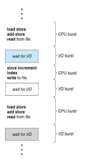
• A process execution cycle alternates between:
  • CPU burst – when the process uses the CPU.
  • I/O burst – when the process waits for I/O operations.
• The final CPU burst usually ends with a system call to terminate execution.

CPU Scheduling Overview

• CPU Scheduling optimizes process execution order for better system performance.
• The short-term scheduler selects a process from the ready queue and allocates the CPU to it.
• Scheduling decisions occur when a process:
  1. Switches from running -> waiting
  2. Switches from running -> ready
  3. Switches from waiting -> ready
  4. Terminates

Scheduling Types

Type	Description
Preemptive	CPU can interrupt and switch to another process before completion
Non-preemptive	Process retains CPU until it releases it voluntarily

Preemption

• Definition: Temporarily removing a process from the CPU in favor of another (e.g., higher priority or shorter job).
• Used to improve responsiveness and ensure fair CPU distribution.

Non-Preemptive vs Preemptive Scheduling

Aspect	Non-Preemptive	Preemptive
CPU Allocation	Process keeps CPU until completion or I/O wait	CPU assigned for a limited time
Interrupt	Process runs until it voluntarily releases CPU	Can interrupt a process at anytime
Overhead	Low (No overhead of switching mid-execution)	High (due to context switching)
Starvation	Possible if long jobs block short ones	Possible if high-priority tasks frequently arrive
Synchronization	Easier	Complex with shared data and kernel activities
Flexibility	None; cannot interrupt current task	Flexible; can prioritize urgent processes
CPU Utilization	Lower	Higher
Waiting Time	Higher	Lower
Response Time	Slower	Faster, but risk of race conditions
Examples	FCFS, Shortest Job First	Round Robin, Shortest Remaining Time First

Dispatcher

• The dispatcher transfers CPU control to the selected process.
  Steps:
  1. Context switch
  2. Switch to user mode
  3. Jump to the user program's next instruction
• Dispatch latency: the time required to stop one process and start another.

Scheduling Criteria

Metric	Description	Goal
CPU Utilization	Keep CPU busy	Maximize
Throughput	Number of processes completed per unit time	Maximize
Turnaround Time	Total time from submission to completion	Minimize
Waiting Time	Time spent waiting in the ready queue	Minimize
Response Time	Time from request submission until first response	Minimize

Scheduling Algorithm Formulas

• Turnaround Time = Completion Time − Arrival Time
• Waiting Time = Turnaround Time − Burst Time
• Throughput = Total Processes / Total Completion Time

Scheduling Algorithms

1. First-Come, First-Served (FCFS)
2. Shortest Job First (SJF)
3. Priority Scheduling
4. Round Robin (RR)
5. Multilevel Queue Scheduling
6. Multilevel Feedback Queue Scheduling

First-Come, First-Served (FCFS)

• Processes are executed in order of arrival (FIFO queue).
• Process Control Block (PCB) added to queue tail upon arrival.
• When CPU is free, process at the head gets executed.
• Simple to implement but inefficient for varying burst times.

Example

Process	Burst Time
P1	24
P2	3
P3	3

Order: P1 -> P2 -> P3
Average Waiting Time = (0 + 24 + 27)/3 = 17
Gantt Chart:

| P1 |------------------------| P2 |---| P3 |---|
0    24                       27   30

Reordered (P2, P3, P1): Average Waiting Time = 3

Drawback: Convoy effect – long processes delay short ones.

Advantages and Disadvantages

Advantages	Disadvantages
Easy to implement	High waiting time for short processes
Fair (no starvation)	Poor CPU utilization

2. Shortest Job First (SJF)

Concept

• Each process is associated with the length of its next CPU burst.
• The process with the shortest burst time is scheduled next.
• Optimal for minimizing average waiting time but requires burst prediction.

Burst Length Prediction

$${\tau }_{n+1}=\alpha t_n+(1-\alpha ){\tau }_n$$

Where:

• ${\tau }_{n+1}$: predicted burst time for next cycle
• $t_n$: actual burst time for current cycle
• $\alpha$: smoothing factor ($0<=\alpha <=1$), often 0.5

Advantages

• Efficent and minimizes average waiting time.

Disadvantages

• Difficult to predict burst length.
• Starvation possible for longer processes.

3. Shortest Remaining Time First (SRTF)

• Preemptive version of SJF.
• Chooses process with the least remaining CPU burst time.

Advantages

Lower average waiting time than non-preemptive.

Disadvantages

• Complex to estimate burst times.
• Risk of starvation and excessive context switches.

4. Priority Scheduling

Concept

• Each process has a priority number; lower numbers indicate higher priority.
• The CPU is allocated to the highest-priority process.
• Can be preemptive or non-preemptive.
• SJF is a special case of priority scheduling where priority = 1 / (next CPU burst time).

Issues

• Starvation: low-priority processes may never execute.
• Solution: Aging – increase process priority the longer it waits.

Example

Process	Burst	Priority
P1	10	3
P2	1	1
P3	2	4
P4	1	5
P5	5	2

Average Waiting Time ≈ 8.2 ms

Advantages

• Flexibility based on importance

Disadvantages

• Starvation of low-priority jobs
• Complex to manage dynamically

5. Round Robin (RR)

Concept

• Each process gets a fixed time quantum (q) (10–100 ms typical).
• After the quantum expires, the process is preempted and placed at the end of the ready queue.
• Suitable for time-sharing systems.

Example (q = 4)

Process	Burst Time
P1	24
P2	3
P3	3

Order: P1 -> P2 -> P3 -> P1 -> …
Average Waiting Time = 3.6 ms

Formulas

• Turnaround Time: End Time - Arrival Time
• Waiting Time: Turnaround Time - Burst Time

Characteristics

• Fairness: all processes get CPU time, no starvation.
• Performance depends on quantum size:
  • Large q -> behaves like FCFS.
  • Small q -> high overhead due to frequent context switches.

Comparison of Scheduling Algorithms

• Preemptive algorithms yield better performance, but risk starvation.
• FCFS is simplest but performs poorly for interactive systems.
• Round Robin ensures fairness and avoids starvation in time-shared systems, but depends heavily on quantum size.

Multilevel Queue Scheduling

• Ready queue divided into multiple queues.
• Each queue has its own scheduling algorithm:
  • Foreground (interactive) -> Round Robin
  • Background (batch) -> FCFS

Scheduling Between Queues

• Fixed Priority: serve all foreground before background (risk of starvation).
• Time Slice: allocate CPU time proportionally (e.g., 80% to foreground, 20% to background).

Multilevel Feedback Queue Scheduling

• Processes can move between queues based on behavior and aging.

• Implements aging to prevent starvation.

• Parameters:

  • Number of queues
  • Scheduling per queue
  • Promotion/demotion policies
  • Queue entry rules

Example:

Queue	Algorithm	Time Quantum
Q0	Round Robin	8 ms
Q1	Round Robin	16 ms
Q2	FCFS	–

Evaluation of Scheduling Algorithms

Evaluation methods help determine the most effective algorithm per use case.

1. Deterministic Modeling

• Evaluates performance for fixed workloads.
• Simple, fast, but only valid for specific input values.

2. Queueing Models

• Represents system as a network of queues (CPU, I/O).
• Uses Little's Formula:$$n=\lambda \times W$$
  • n: average number of processes in queue
  • λ: arrival rate
  • W: average waiting time

3. Simulation

• Emulates system behavior using random input or real trace data.
• Allows more accurate, flexible analysis.

4. Implementation

• Most accurate but costly and environment-dependent.
• Requires modifying and testing the OS itself.
• Environment and workload variations affect results.